Участник:АРыбников/Песочница

Априорная теория всего

физика

монография

Песочница

Автор:

Александр Рыбников

• Теория всего не от мира сего

Дата написания:

24 сентября 2023 года

Язык оригинала:

русский

Оригинал:

Теория всего не от мира сего

Предмет:

Решётчатая модель пространства-времени

https://proza.ru/avtor/alrybn1946

	Behind it all is surely an idea so simple, so beautiful, that when we grasp it - in a decade, a century, or a millennium - we will all say to each other, how could it have been otherwise? How could we have been so stupid?
— John Archibald Wheeler

Definition

A theory of everything — a physical-mathematical theory, all known variants of which have been carefully examined and rejected, now looks completely unexpected and fundamentally different from all previous versions.

	The a priori theory of everything is the most detailed self-realizing project of the Metaverse, up to stars as self-forming, self-functioning, and self-removing thermonuclear reactors.
— Aleksandr Rybnikov, author

In essence, the a priori theory of everything is the primary term of this theory and creates a naturally unified basis for the interpretation of cosmology, which studies the properties and evolution of the Metaverse as a whole, which is inaccessible to humanity in space and time. Hence, such a theory has no prototypes or variants in principle, because it is itself the only prototype. It comes at once and completely from a brief source, which, due to the above, is not written in any common language.

The latter means that the content of the a priori theory of everything arises as a result of the interpretation of the axiom, formulated as a mathematical formula. Its interpretation in the silence of the ages was done by mathematicians and physicists.

No Big Bangs, hundreds of inflations or Sinai in flames, shrouded in thick smoke; trembling earth; thundering thunder; flashing lightning; and in the noise and bedlam, covering it, the voice of God, uttering commandments (Ex. 19:1 and following). Nothing like this ever happened and could not happen in principle. No popular version of the stable functioning of the Metaverse will ever be written because of the mathematical formula underlying it.

Therefore, the goal of the a priori theory of everything is to build as long as possible a mathematical chain of consequences from the original axiom, including the exposition of cosmology. Thus, the interpretation introduces the relationship of the a priori axiom with the consequences observed in practice, that is, translates the original mathematical concepts of the axiom into physical language. The need to accept the axiom of existence without proof follows only from an inductive consideration: any proof is forced to rely on some statements and the chain will be infinite if you require your proofs for each of them. Nevertheless, explicit experimental evidence at the level of space and time, fundamental interactions, and elementary particles exist and they ‘break the infinite’. Thanks to this, it is always possible and necessary to go beyond the edge, to accept the challenges of developing physics.

In the a priori theory of everything, the question of the truth of the axiom of existence was solved almost 300 years ago.

Chronicles of the A Priori Theory of Everything

Leonhard Euler

From a distance, everything looks different.

Therefore, it can be said that on May 16 (27), 1703, at the mouth of the Neva River, Saint Petersburg was founded for the very purpose of creating an a priori theory of everything. On this day, Tsar Peter I laid the foundation of the Peter and Paul Fortress on the city’s first structure, Hare Island. Internal transformations and military victories in the Great Northern War contributed to the transformation of Russia into an Empire, which was officially proclaimed on October 22 (November 2), 1721, when, at the request of the senators, Peter I assumed the titles of Emperor of All Russia and Father of the Fatherland. Just a few years later, by imperial decree on January 22 (February 2), 1724, the Academy of Sciences and Arts was established in Saint Petersburg.

Subsequently, an edict by Empress Catherine I on February 23 (March 6), 1725, invited scholars to the Russian Academy of Sciences and provided the necessary support for those wishing to travel to Russia. In the early winter of 1726, Leonhard Euler (born April 15, 1707, Basel, Switzerland – died September 7 (18), 1783, Saint Petersburg, Russian Empire) received news from Saint Petersburg: based on the recommendation of the Bernoulli brothers, he was invited to the position of adjunct in the rapidly growing capital of the new world empire. His work in Saint Petersburg was so fruitful that it caught the attention of Russophobes:

	In mathematics, it is customary to name a discovery after the second person who made it, otherwise, everything would have to be named after Euler
— a humorous folk rule.

In particular, Euler continued research on the connection between the constant $\pi$ as a symbol of implicit $\infty$ and the constant $\ e$ as a symbol of explicit $\infty$, where Euler’s number $\ e$ — one of the most important mathematical constants — can be expressed as follows: $$\begin{equation*}\boxed{\ e = \sum_{n=0}^{\infty} \frac{1}{n!}. }\end{equation*}$$

The investigation of this connection began in 1714 with the publication of Euler’s formula, which asserts that for any real number $\varphi$, the following equality holds:

The geometric interpretation of Euler’s formula

$$\begin{equation*} \boxed{\ e^{i\varphi}=\cos \left(\varphi\right) +i\sin \left(\varphi\right).}\end{equation*}$$ This formula establishes a profound link between exponential functions, trigonometry, and complex numbers. It unifies these seemingly distinct mathematical concepts and plays a fundamental role in various fields of mathematics and physics. From here, when $\varphi=\pi$, Euler’s identity emerges, connecting five fundamental mathematical constants: $$\begin{equation*} \boxed{\ e^{i\pi}+1=0. }\end{equation*}$$

This remarkable equation unites the exponential function $\ e$, the imaginary unit $\ i$, the transcendental number $\pi$, the additive identity $0$, and the multiplicative identity $1$. It stands as a testament to the elegance and interconnectedness of mathematical concepts.

As a result, he made a fundamental contribution to the a priori theory of everything: in 1729, Leonhard Euler calculated the so-called “nonelementary antiderivative” integral: $\begin{equation} \label{axiom} \boxed{\frac{1}{\sigma\sqrt{2\pi}}\int_{-\infty}^{\infty}\ e^{-\frac{1}{2}(\frac{x}{\sigma})^{2}}dx=1.}\end{equation}$ This integral plays a crucial role in probability theory, statistics, and various scientific fields. Euler’s work continues to shape mathematical and scientific research to this day. Please, remember forever that the integral of the normal distribution was specifically calculated by Euler!

It should be noted that the mathematical meaning of this integral was clarified in 1929, when Bruno de Finetti (born on June 13, 1906, in Innsbruck; died on July 20, 1985, in Rome) introduced the concept of an infinitely divisible distribution. Such a distribution describes a random variable that can be represented as an arbitrary number of independent and identically distributed summands.

This marked a complete departure from Gauss’s idea, who believed that his theory only considered a single quantity.

James Clerk Maxwell

The role of Maxwell in the history of physics is not fully understood due to the fact that his equations represent the terms of the first order in an expansion with respect to the fine-structure constant. Thus, Maxwell created the quantum theory of electromagnetic radiation, which was the first theory to describe electricity, magnetism and light as different manifestations of the same phenomenon.

The next part of the history of the a priori theory of everything is a purely mathematical introduction of displacement current into Maxwell’s equations. Or, in modern terms, the introduction of magnetic monopoles.

Perhaps this is the first work in the history of physics where Hegel’s well-known proposition was successfully realized.

	What is reasonable is real; that which is real is reasonable.
— Georg Wilhelm Friedrich Hegel, Elements of the Philosophy of Right

Let’s keep in mind that Maxwell, justifying the mathematical introduction of displacement current, wrote in the language of that time (today such a funny language continues to be used by all sorts of ether worshipers). However, as a result of the development of his theory, Maxwell changed his understanding and abandoned the ether in favor of the displacement current.

So, under the influence of Faraday’s and Thomson’s ideas, Maxwell came to the conclusion that magnetism has a vortex nature, and the electric current - translational. For a vivid description of electromagnetic effects, he created a new, purely naive, mechanical model, according to which rotating “molecular vortices” produce a magnetic field, while the smallest transfer “idle wheels” provide rotation of vortices in one direction. The translational movement of these transfer wheels (“particles of electricity”, in Maxwell’s terminology) ensures the formation of an electric current. At the same time, the magnetic field, directed along the axis of rotation of the vortices, turns out to be perpendicular to the direction of the current, which found expression in the “screw rule” justified by Maxwell.

Within the framework of this mechanical model, Maxwell was able not only to give an adequate visual illustration of the phenomenon of electromagnetic induction and the vortex nature of the field generated by the current, but also to introduce an effect symmetrical to Faraday’s: changes in the electric field (the so-called displacement current, created by shifting the transfer wheels, or associated molecular charges, under the action of the field) should lead to the emergence of a magnetic field. The displacement current directly led to the continuity equation for the electric charge, that is, to the idea of open currents (previously all currents were considered closed). Considerations of symmetry of equations in this, apparently, did not play any role. The famous physicist J. J. Thomson called the discovery of the displacement current “Maxwell’s greatest contribution to physics”. These results were set out in the article “On physical lines of force”, published in several parts in 1861-1862.

In the same article, Maxwell, moving on to considering the propagation of disturbances in his model, noted the similarity of the properties of his vortex medium and Fresnel’s light-bearing ether. This found expression in the practical coincidence of the speed of propagation of disturbances (the ratio of the electromagnetic and electrostatic units of electricity, defined by Weber and Rudolf Kohlrausch) and the speed of light, measured by Hippolyte Fizeau. Thus, Maxwell made a decisive step towards the construction of the electromagnetic theory of light:

	We can hardly refuse to conclude that light consists of transverse oscillations of the same medium that is the cause of electrical and magnetic phenomena.
— James Clerk Maxwell

However, this medium (ether) and its properties were not of primary interest to Maxwell, although he certainly shared the view of electromagnetism as a result of applying the laws of mechanics to the ether:

	Maxwell does not give a mechanical explanation of electricity and magnetism; he limits himself to proving the possibility of such an explanation.
— Henri Poincaré

In 1864, Maxwell published the article “A Dynamical Theory of the Electromagnetic Field,” in which he gave a more detailed formulation of his theory (the term “electromagnetic field” appeared here for the first time). In doing so, he discarded the crude mechanical model (such representations, according to the scientist, were introduced exclusively “as illustrative, not as explanatory”), leaving a purely mathematical formulation of the field equations (Maxwell’s equations), which for the first time were treated as a physically real system with a definite energy. In the same work, he effectively proposed the hypothesis of the existence of electromagnetic waves, although, following Faraday, he wrote only about magnetic waves (electromagnetic waves in the full sense of the word appeared in the 1868 article). The speed of these transverse waves, according to his equations, is equal to the speed of light, and thus the concept of the electromagnetic nature of light was finally formed. Moreover, in the same work, Maxwell applied his theory to the problem of the propagation of light in crystals, the dielectric or magnetic permeability of which depends on the direction, and in metals, obtaining a wave equation taking into account the conductivity of the material.

Thus, the most important contribution to the concept of the theory of everything was made by Maxwell in the work “On Physical Lines of Force,” consisting of four parts and published in 1861-1862, in which the necessity of introducing a fundamentally new concept of displacement current was shown. Generalizing Ampère’s law, Maxwell introduces the displacement current, probably to link currents and charges by the continuity equation, which was already known for other physical quantities. Therefore, in this article, the formulation of the complete system of electrodynamics equations was essentially completed. In the 1864 article “A Dynamical Theory of the Electromagnetic Field,” the previously formulated system of 20 equations for 20 unknowns was considered. In this article, Maxwell first formulated the concept of the electromagnetic field as a physical reality, having its own energy and finite propagation time, determining the delayed nature of electromagnetic interaction.

Some physicists opposed Maxwell’s theory (especially many objections were raised by the concept of displacement current). Helmholtz proposed the own theory, a compromise relative to the models of Weber and Maxwell, and entrusted his student Heinrich Hertz to conduct its experimental verification. However, Hertz’s experiments unequivocally confirmed the correctness of Maxwell.

Arnold Sommerfeld

The need to write this chapter is due to the fact that it marks the end of the period of spontaneous approaches to the a priori theory of everything and the beginning of its crystallization. In natural science, such moments mature regularly and scientists themselves overcome them more or less painlessly. It should be noted that the damned secret of physics does have Russian roots, as its creator was born and studied in the semi-exclave of the Kaliningrad region of Russia (like Alaska for the USA). In 1891, Arnold Sommerfeld defended his doctoral dissertation in Kaliningrad (then still Königsberg) and then settled in Munich in search of work.

In 1913, Sommerfeld became interested in the research of the Zeeman effect, which was being conducted by the famous spectroscopists Friedrich Paschen and Ernst Back, and attempted to theoretically describe the anomalous splitting of spectral lines based on the generalization of Lorentz’s classical theory. Quantum ideas were used only to calculate the intensities of the splitting components. In July 1913, the famous work of Niels Bohr was published, which contained a description of his atomic model, according to which an electron in an atom can rotate around the nucleus along so-called stationary orbits without emitting electromagnetic waves. Sommerfeld was well acquainted with this article, a copy of which he received from the author himself, but at first he was far from using its results, having a skeptical attitude towards atomic models as such. Nevertheless, already in the winter semester of 1914-1915, Sommerfeld read a course of lectures on Bohr’s theory, and around the same time, he had thoughts about the possibility of its generalization (including relativistic).

The need for a generalization of Bohr’s theory was associated with the lack of a description of more complex systems than hydrogen and hydrogen-like atoms. In addition, there were small deviations of the theory from experimental data (lines in the spectrum of hydrogen were not truly single), which also required explanation. In one of the reports of the Bavarian Academy of Sciences and in the second part of his large article "On the Quantum Theory of Spectral Lines" (Zur Quantentheorie der Spektrallinien, 1916), Sommerfeld presented a relativistic generalization of the problem of an electron moving around the nucleus along an elliptical orbit, and showed that the perihelion of the orbit in this case slowly precesses. Sommerfeld managed to obtain a formula for the total energy of the electron, which included an additional relativistic term, determining the dependence of energy levels on both quantum numbers separately. As a result, the spectral lines of a hydrogen-like atom should split, forming the so-called fine structure, and the dimensionless constant introduced by Sommerfeld, the fine structure constant $\alpha$ (FSC), determined the magnitude of this splitting. Precision measurements of the spectrum of ionized helium, conducted by Friedrich Paschen in the same year of 1916, confirmed Sommerfeld’s theoretical predictions.

The constant $\alpha$ in the SI system of units can be defined as follows: $$\begin{equation} \label{alpha} \boxed{\alpha=\frac{e^2}{\ 4 \pi \varepsilon_0 \hbar c}=\frac{e^2}{2 \varepsilon_0 h c}}\end{equation},$$ where e is the charge of an electron, ε₀ is the permittivity of free space, ħ is the reduced Planck constant and c is the speed of light.

The success in describing the fine structure was a testament in favor of both Bohr’s theory and the theory of relativity and was enthusiastically accepted by a number of leading scientists.

	Your spectral studies are among the most beautiful things I have experienced in physics. Thanks to them, Bohr’s idea becomes completely convincing.
— Einstein

In his Nobel lecture (1920), Planck compared Sommerfeld’s work with the theoretical prediction of the planet Neptune. However, some physicists (especially those anti-relativistically inclined) considered the results of the experimental verification of the theory unconvincing. A strict derivation of the fine structure formula was given by Paul Dirac in 1928 based on a consistent quantum-mechanical formalism, so it is often called the Sommerfeld-Dirac formula. This coincidence of results, obtained within the framework of Sommerfeld’s semi-classical method and with the help of Dirac’s rigorous analysis (taking into account spin!), was interpreted differently in the literature. Perhaps the reason for the coincidence lies in an error made by Sommerfeld and turned out to be very handy. Another explanation is that in Sommerfeld’s theory, the neglect of spin successfully compensated for the lack of a rigorous quantum-mechanical description. Such a detailed description of the vicissitudes of the appearance of the FSC is given because at this time the First World War was already in full swing - one of the two most powerful and most terrible armed conflicts in human history. After the end of the First World War, the development of all physics accelerated. First of all, this concerned the discovery of new fundamental interactions, which at first glance no longer had anything in common with Maxwell’s equations. Thus, the original goal was finally lost - the description based on Maxwell’s equations of both space and time itself, and all fundamental interactions, as well as the existence of fundamental elementary particles. Subsequently, in quantum electrodynamics, the fine structure constant $\alpha$ acquired the value of the interaction constant, characterizing the intensity of interaction between electric charges and photons.

Paul Dirac

The next important step towards creating a theory of everything was made by Dirac in 1931 in the article “Quantized Singularities in the Electromagnetic Field”, where he introduced the concept of a magnetic monopole, whose existence could explain the quantization of electric charge. Later, in 1948, he returned to this topic and developed a general theory of magnetic poles, considered as ends of unobservable strings. Since then, magnetic monopoles have firmly entered modern physics.

For the a priori theory of everything, the idea of the magnetic monopole introduced by Dirac is fundamentally important, and the relationship between the magnitudes of the magnetic and electric charge established in his article is: $$\begin{equation} \label{monopol} \boxed{\frac{q_{S}}{q_{e}}=\frac{q_{N}}{q_{p}}=\frac{1}{2\alpha},}\end{equation},$$ where $q_{S}$ and $q_{N}$ are the charges of the Dirac magnetic monopole, $q_{e}$ is the charge of the electron, and $q_{p}$ is the charge of the positron. Since the denominators contain the charges of the particle and antiparticle, it can be expected that the numerators also contain the charges of the particle and antiparticle!

From the perspective of the theory of everything, this idea has advanced physics so much that even Dirac himself could not fully appreciate its consequences. In fact, a similar situation occurred a few years earlier when Dirac predicted the positron and proposed the idea of the “Dirac sea”.

Unfortunately, the fundamentally incorrect idea of particle birth and annihilation attracted more attention than the correct idea of the magnetic monopole. It is unlikely that Dirac himself was fully responsible for it in the sense that energy can create the mass of any particle. However, Dirac did say something about the existence of ready positrons in the “Dirac sea”! Followers of the idea of particle birth and annihilation applied it directly to the vacuum, behind which the ether, rejected by Maxwell, clearly emerged!

Nevertheless, after the prediction of antiparticles and their successful experimental confirmation, finding a magnetic monopole was not as quick. For a trivial reason. No one understood the essence of the formula, which stated that the intensity of interaction of magnetic monopoles significantly exceeds the intensity of interaction of electric charges! This meant that no means available to experimenters could register a magnetic monopole.

Indeed, Dirac himself added fuel to the fire.

	It seems that one of the fundamental properties of nature is that the basic physical laws are described by a mathematical theory with such elegance and power that an extremely high level of mathematical thinking is required to understand it. You may ask: why is nature arranged this way? The only answer is that our modern knowledge shows that nature is apparently arranged in this way. We just have to agree with it. Describing this situation, one could say that God is a mathematician of a very high class, and in constructing the Universe, He used very complex mathematics.”
— P. A. M. DiracProperty "Цитата/Автор" (as page type) with input value "— P. A. M. Dirac[3]" contains invalid characters or is incomplete and therefore can cause unexpected results during a query or annotation process.

As a result, most physicists declared Dirac’s magnetic monopoles hypothetical particles.

Later, in 1948, he returned to this topic and developed it into a more general concept of a non-local particle considered as the ends of an unobservable “string” for displacement current. Since then, magnetic monopoles have firmly entered modern physics as current-carrying particles. As if both in one bottle.

Unfortunately, he did not unequivocally express this idea. Therefore, Dirac’s magnetic monopoles were developed into the idea of dyons (or diions) by J. Schwinger in 1969. Schwinger introduced the dyon as a particle representing an electrically charged magnetic monopole.

And thousands of physicists, trained exclusively for the nuclear project, began to produce very expensive and high-quality junk at a tremendous speed. In addition to electromagnetic and gravitational interactions, contrived ones appeared: the so-called weak and strong. To these non-existent interactions, non-existent particles were also invented. And this direction of physics ended with the big bang dummy, which has no more intellect than a big mac!

	$\mathrm{N}\!\!\mathrm{B}$ Unfortunately, Dirac himself did not explicitly state that the magnetic monopole he introduced is the carrier of the strongest interaction. Perhaps for him, it was so obvious that he did not dare to tell experimenters that “a magnetic monopole can only be observed with another magnetic monopole.” Accordingly, he did not present the trivial consequence of the strongest interaction — the formation of a crystal from its carriers. On the other hand, if Dirac had explicitly said this, physics could have done without the “strong interaction” of H. Yukawa, quarks, and much more.
— Aleksandr Rybnikov, author

Mathematical Foundations of Obtaining a Fine Structure Constant

	It's one of the greatest damn mysteries of physics: a magic number that comes to us with no understanding by man. You might say the "hand of God" wrote that number, and "we don't know how He pushed his pencil." We know what kind of a dance to do experimentally to measure this number very accurately, but we don't know what kind of dance to do on the computer to make this number come out, without putting it in secretly!
― Richard P. FeynmanProperty "Цитата/Автор" (as page type) with input value "― Richard P. Feynman[4]" contains invalid characters or is incomplete and therefore can cause unexpected results during a query or annotation process.

As always, the experimenters were against it. They were fishing in murky waters, trying to detect the heterogeneity of the fine-structure constant in time or space. As a result, the relevance of searching for a mathematical formulation of the FSC fell by the wayside.

Intensity of interactions

If we choose an object that participates in all fundamental interactions, then the values of the dimensionless constants of these interactions, found by the general rule, will show the relative intensity of these interactions. The proton is most often used as such an object at the level of elementary particles. The basic energy for comparing interactions is the electromagnetic energy of a photon, which is defined as: $$U_f= \frac{h c}{\lambda}.$$ The choice of photon energy is not random, as the wave representation, based on electromagnetic waves, lies at the heart of modern physics. With their help, all basic measurements are made — lengths, times, and including energy.

Spatial Hyperanalytic Function

Idea

It is known that there is a fundamental relationship between the analyticity of a function and the rate of decay of its Fourier coefficients.

The better the function, the faster its coefficients tend to zero, and vice versa. Power decay of Fourier coefficients is inherent in polynomials, and exponential decay is inherent in analytic functions. However, it turns out that the generating function for the FSC does not belong to the specified types of functions, as a distinctive feature of the mathematical equations of quantum mechanics is the presence in them of the symbol of Planck’s constant. Hence follows the possibility of the existence of hyperanalytic functions, for which the decay of Fourier coefficients corresponds to tetration.

In addition, it should be clarified that, unlike traditional physics, the a priori theory of everything unexpectedly considers two types of fundamental interactions: spatial and temporal.

Definition of Spatial Hyperanalytic Function (SHF)

	The integral itself $\left(\ref{axiom}\right)$ is useless since it is not taken. As is known, there is no chance to find the keys lost at night somewhere. They should be looked for exactly under the lamp. Spatial fundamental interactions are manifested in the decomposition of the spatial lattice function $\mathbb{R}\left(x\right)$. $$\boxed{\frac{1}{\sigma\sqrt{2\pi}}\int_{-\infty}^{\infty}e^{-\frac{1}{2}(\frac{x}{\sigma})^{2}}dx=\frac{1}{\sigma\sqrt{2\pi}}\int_{-\frac{L}{2}}^{\frac{L}{2}}\sum_{n=-\infty}^{\infty}e^{-\frac{1}{2}(\frac{x-nL}{\sigma})^{2}}dx=1.}$$ This is where Euler’s dream comes from: quantification of monotonic exponential functions turns them into oscillatory trigonometric functions: $$\begin{equation} \label{hiper} \boxed{\mathbb{R}(x)=\frac{1}{\sigma\sqrt{2\pi}}\sum_{n=-\infty}^{\infty}e^{-\frac{1}{2}(\frac{x-nL}{\sigma})^{2}}.} \end{equation}$$
— Aleksandr Rybnikov, author

Decomposition of SHF

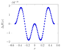
The graphs of the SHF and its components, presented in the gallery, clearly demonstrate that the decrease in Fourier coefficients for hyperanalytic functions corresponds to tetration.

• The graphs of the SHF and its components
• 

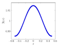
  SHF

• 

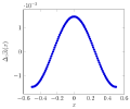
  First Difference of SHF

• 

  Second Difference of SHF

• 

  Third Difference of SHF

• 

  Fourth Difference of SHF

• 

  Fifth Difference of SHF

As mentioned earlier, the deviation of the function $\mathbb{R}\left(x\right)$ from one is of interest. From the SHF graph, it can be seen that the maximum value of SHF is reached when x=0: $$\mathbb{R}\left(0\right)=\mathbb{R}_{max}=\frac{1}{\sigma\sqrt{2\pi}}\sum_{n=-\infty}^{\infty}e^{-\frac{1}{2}\left(\frac{-n}{\sigma}\right)^{2}}.$$

The minimum value of the PRF is reached when x=1/2: $$\mathbb{R}\left(1/2\right)=\mathbb{R}_{min}=\frac{1}{\sigma\sqrt{2\pi}}\sum_{n=-\infty}^{\infty}e^{-\frac{1}{2}\left(\frac{1/2-n}{\sigma}\right)^{2}}.$$

	Let’s introduce the mathematical function of fine structure $\mathbb{\alpha}\left(\sigma\right)$ as the average relative value of the unevenness of the distribution of filling a unit segment by the function $e^{-\frac{1}{2}(\frac{x}{\sigma})^{2}}$, depending on $\sigma$: $$\begin{equation} \label{newtalpha} \boxed{\mathbb{\alpha}\left(\sigma\right)=\frac{1}{2}\frac{\mathbb{R}_{max}-\mathbb{R}_{min}}{\mathbb{R}_{max}+\mathbb{R}_{min}}.}\end{equation}$$
— Aleksandr Rybnikov, author

The choice of the name and designation of the parameter $\mathbb{\alpha}$ is due to the fact that $$\mathbb{\alpha}\left(0.4992619105929628\right)=\alpha.$$ Now everyone knows the solution to the cursed mystery of physics that has existed for more than a hundred years!

Since the distribution of filling a unit square with the function $e^{-\frac{1}{2}(\frac{x}{\sigma})^{2}}$ turns out to be above and below one, a deuce must be present in the definition, just as in formula $\left(\ref{alpha}\right)$. Thus, there are no other mathematical constants in formula $\left(\ref{alpha}\right)$.

The slight difference of $\sigma$ from the natural value of 0.5 will be explained later. Let $A_{0}$ is the constant term of the decomposition of SHF: $$A_{0}=\frac{\mathbb{R}_{max}+\mathbb{R}_{min}}{2}.$$ As a result of subtracting $A_{0}$ from $\mathbb{R}(x)$, we obtain the first difference. The first difference can be approximated as follows: $$A_{1}\left(x\right)=\frac{\mathbb{R}_{max}-\mathbb{R}_{min}}{2} \cos\left(2\pi x\right).$$ Using definition $\left(\ref{newtalpha}\right)$, the first difference can be rewritten as follows: $$A_{1}\left(x\right)=\frac{\mathbb{R}_{max}+\mathbb{R}_{min}}{2}\left(2\alpha\left(\sigma\right)\cos\left(2\pi x\right)\right).$$ Thus, the first term of the generating function containing PTS is obtained. Comparing the obtained formula with the equation $\left(\ref{monopol}\right)$, it becomes clear that the intensity of the magnetic monopole interaction is equal to $\alpha^0$.

Even Differences of SHF Expansion

All subsequent even differences can be called submerged $\overline{\mathbb{V}}\left(2i\times2\pi x\right)$ -functions, which are approximated as follows: $$A_{2i}\left(x\right)=c_{2i}\left(\cos\left(2i\times2\pi x\right)-1\right).$$

where $$\sum_{i=1}^{\infty}c_{2i}=\frac{\mathbb{R}_{max}+\mathbb{R}_{min}}{2}-1=2 * \sum_{k=1}^{\infty} \alpha^{4^{k}}.$$

Using the value $$\mathbb{R}\left(1/4\right)=\mathbb{R}_{1/4}=\frac{1}{\sigma\sqrt{2\pi}}\sum_{n=-\infty}^{\infty}e^{-\frac{1}{2}\left(\frac{1/4-n}{\sigma}\right)^{2}}$$

we define the amplitude for $c_{2}$ $$\frac{1}{2}\left(\frac{\mathbb{R}_{max}+\mathbb{R}_{min}}{2}-\mathbb{R}_{1/4}\right)=2\alpha^{4}.$$

As a result, we get: $$c_{2i}= \alpha^{4^{i}}.$$

Thus, it is for the even differences that a pedestal was added to the unit average value.

Odd Differences of SHF Expansion

It is obvious that no SHF can be analytically decomposed into a Fourier series, as it is not integrated in elementary functions. Because of this, PRF cannot be decomposed into an even and odd function. An arbitrary function $f:[-X,X] \subset \mathbb{R} \to \mathbb{R}$ can be uniquely represented as the sum of an odd and an even function: $$f(x) = g(x) + h(x),$$ $$g(x) = \frac{f(x) - f(-x)}{2},\; h(x) = \frac{f(x)+f(-x)}{2}.$$ The functions $g(x)$ and $h(x)$ are called the odd part and the even part of the function $f(x)$, respectively.

Thanks to this, SHF can be decomposed into an infinite series of primitive hyperanalytic functions (fractals) by successive attempts to decompose PRF into an even and odd function. Thus, SHF can be decomposed into a series in the simplest way, but unlike the orthonormal Fourier series, the obtained series is no longer such.

The odd difference $\mathbb{W}^{\text{odd}}\left((2i-1)\times2\pi x\right)$ is no longer a hyperanalytic function and are equal to: $$\mathbb{W}^{\text{odd}}\left((2i-1)\times2\pi x\right)=\frac{\mathbb{W}\left((2i-1)\times2\pi x\right)-\mathbb{W}\left((2i-1)\times2\pi\left(0.5-x\right)\right)}{2}.$$ It can be approximated with any degree of accuracy as follows $$A(W^{\text{odd}}\left((2i-1)\times2\pi x\right))=\beta (\cos\left(3(2i-1)\times2\pi x\right)- \cos\left((2i-1)\times2\pi x\right)),$$ where $\beta$ is a normalization factor. The function $\mathbb{W}\left((2i-1)\times2\pi x\right)$ should be decomposed into an even and odd difference. Its even difference is equal to: $$\mathbb{W}^{\text{even}}\left((2i-1)\times2\pi x\right)=\frac{\mathbb{W}\left((2i-1)\times2\pi x\right)+\mathbb{W}\left((2i-1)\times2\pi\left(0.5-x\right)\right)}{2},$$ as can be seen from the graphs.

Аппроксимация SHF

Now the approximation $\mathbb{R}(x)$ will take the form:

$$\begin{equation} \label{allinone} \begin{aligned} A\left(x\right)=\frac{\mathbb{R}_{max}+\mathbb{R}_{min}}{2}(1+2\alpha \cos\left(2\pi x\right))\\ +2\sum_{i=1}^{\infty}\alpha^{4^{i}}\left(\cos\left(2i\times 2\pi x\right)-1\right)\\ +\frac{2}{\mathbb{W}_{max}}\sum_{i=1}^{\infty}\alpha^{9{i}²}\left(\cos\left(3 \times (2i-1)\times 2\pi x\right)-\cos\left((2i-1) \times 2\pi x\right)\right), \end{aligned}\end{equation}$$ where $\mathbb{W}_{max}$ is a normalization factor equal to the value of the sum at the maximum point. The coefficient 2 for all cosines is a consequence of the symmetry of $\mathbb{R}(x)$ with respect to x=0.

	$\mathrm{N}\!\!\mathrm{B}$ It’s just amazing how simple the equation of a star as a nuclear reactor is.
— Alexandr Rybnikov, author

Approximation of the Three-Dimensional SHF

The three-dimensional $\mathbb{R}\left(x,y,z\right)$ can be obtained from its one-dimensional definition: $$\mathbb{R}\left(x,y,z\right)=\mathbb{R}_{max}^{2}\mathbb{R}\left(x\right).$$

Thus, the approximation of the three-dimensional PRF is also a series from PTS along any axis of the three-dimensional lattice space, and the PTS itself is a function of the dimensionless parameter σ, equal to the ratio of the ‘diameter’ of some physical object located in each cell to the lattice step L. The appearance of the constant fine structure $\mathit{\alpha}$ in the decomposition of the hyperanalytic lattice function is due to the periodicity of space. The periodicity of space is described by a symmetric function of x."

Temporal Hyperanalytic Function

Idea

To obtain the temporal hyperanalytic function (TНF) $\mathbb{R}\left(t\right)$, the direct use of the lattice idea is too trivial. This is because in the case of space, movements in the lattice are possible in any direction, but in the case of time, movements in the lattice are possible only in one direction. The physics of the last century actually came to understand such an idea of time, but did not formulate it mathematically clearly. So, for the first time, the terms boson and fermion were used by Dirac in the lecture ‘Development of Atomic Theory’, read by him on Tuesday, December 6, 1945, at the Paris Science Museum ‘Palace of Discoveries’. The function $\mathbb{R}\left(x\right)$ describes exclusively bosons: states in all nodes of the lattice can be identical. But the function $\mathbb{R}\left(t\right)$ describes exclusively fermions and obeys Fermi-Dirac statistics: no more than one particle can be in one quantum state (Pauli exclusion principle). Thus, it turns out that the Pauli exclusion principle is equivalent to Heisenberg’s uncertainty principle.

	$\mathrm{N}\!\!\mathrm{B}$ Therefore, the concept of time can only be applied to fermions as a transaction - a minimal logically meaningful operation, which makes sense and can only be performed completely. In other words, the idea of time in physics is realized by introducing a lock, which is set before the completion of the disturbance processing. In other words, before the completion of the disturbance processing. And bosons do not have time because they are agents of the transaction. Hence it follows that the second equation should traditionally be called the equation for delayed neutrons. Interestingly, mathematicians have long understood this and use the prediction-correction method to solve the Cauchy problem.
— Alexandr Rybnikov, author

Furthermore, as in the case of three-dimensional space, it is possible to generalize the obtained decomposition to three-dimensional time since there are no formal restrictions for a similar generalization.

Definition of THF

As a “lock” on movements in forbidden directions, it is advisable to use the definition of the derivative of the normal distribution over time, but without taking the limit.

Let $\mathbb{R}\left(t\right)$ be a THF on the unit interval $\left[-T/2, T/2\right]$ with $\tau=\sigma$ and $T=1$: $\begin{equation} \label{time}\boxed{\mathbb{R}\left(t\right)=\frac{1}{\tau\sqrt{2\pi}}\sum_{i=-\infty}^{\infty}\left[ \exp\left(-\frac{1}{2}\left(\frac{t+T/4-iT}{\tau}\right){2}\right)-\exp\left(-\frac{1}{2}\left(\frac{t-T/4-iT}{\tau}\right){2}\right)\right].} \end{equation}$

The graphs of THF and its components, presented in the gallery, clearly demonstrate that the decay of the Fourier coefficients for the hyperanalytic function $\mathbb{R}\left(t\right)$ corresponds to tetration.

• The graphs of the THF and its components
• 

  THF

• 

  First difference of THF

• 

  Second difference of THF

• 

  Right-left time course

By successively subtracting the sines from $\left(\ref{time}\right)$, it can be shown that the approximation of $\mathbb{R}\left(t\right)$ has the following form:

$\begin{equation} A\left(t\right)=\sum_{k=0}^{\infty}\left(-1\right)^{k+1}a_{k} \sin\left(2\pi\left(2k+1\right)t\right). \end{equation}$ “To determine the values of the coefficients $a_{k}$, we use $k+1$ equations with different values of $l$: $$\sum_{i=0}^{k}\left(-1\right)^{i}a_{i} \sin\left(\frac{2i+1}{2l+1}\frac{2\pi}{4}\right) = \mathbb{R}\left(\frac{1}{4\left(2l+1\right)}\right).$$

Given that $A\left(1/4\right)$ is numerically equal to $$2\left(\mathbb{R}_{max}\left(\tau\right)+\mathbb{R}_{min}\left(\tau\right)\right)\alpha\left(\tau\right),$$ the equation $\left(\ref{time}\right)$ can be written in the following form: $$\begin{equation} \label{delayed}\boxed{ \alpha_{eff}\left(t,\tau\right) = -\alpha \sin\left(2\pi t\right) + \sum_{k=1}^{\infty}\left(-1\right)^{k+1}\sqrt{\left(2k+1\right)}\alpha^{2((2k+1)^{2})} \sin\left(2\pi\left(2k+1\right)t\right).}\end{equation}$$

The appearance of $\alpha$ in the decomposition of the hyperanalytic THF $\mathbb{R}\left(t\right)$ is also a hyperanalytic function.

What $\alpha$ are we measuring?

The equation $\left(\ref{delayed}\right)$ raises an interesting question about the real value of the fine-structure constant.

Features of THF

One-dimensional time can be generalized to three-dimensional right-left time of a fermion particle, in which the transition forward or backward along the time axis is combined with a right or left turn in time by 180 degrees.

The need for such a generalization is due to the fact that from $\left(\ref{delayed}\right)$ follows: $\sin \left(2\pi t\right)\simeq-\frac{\alpha_{eff}\left(t,\tau\right)}{\alpha}.$

At the same time, from the definition of $\mathbb{R}\left(t\right)$ $\left(\ref{time}\right)$ it can be seen that the lowest frequency pair is approximated as follows: $$\sin \left(\pi t\right)\simeq- m\left[\exp \left(-\frac{1}{2}\left(\frac{t+1/4}{\tau}\right)^{2}\right)-\exp \left(-\frac{1}{2}\left(\frac{t-1/4}{\tau}\right)^{2}\right)\right],$$ where m is a normalization factor. From this, it can be seen that the actual local frequency $\mathbb{R}\left(t\right)$ is twice as small as the observed group frequency $\alpha_{eff}$. In addition, generalization to right-left time allows us to see that the change in $\mathbb{R}\left(t\right)$ over time is actually due to both movement along the t-axis and simultaneous rotation near this axis.

A graphical illustration of this hypothesis is shown in the figure “Course of right-left time”.

Features of THF Calculation

Despite the fact that there is no time derivative as such in the lattice space, the predictor-corrector method for the Cauchy problem, developed by Euler in 1768, needs to be applied to solve the equation $\left(\ref{delayed}\right)$. Thus, the living spirit manifests itself even when eliminated.

Equations of the Eternal Thermonuclear Reactor

Idea

English Wikipedia, violating the neutrality rule, asks:

	Is string theory, superstring theory, or M-theory, or some other variant on this theme, a step on the road to a "theory of everything", or just a blind alley?
— Wikipedia, Theory of everything

	$\mathrm{N}\!\!\mathrm{B}$ As it turned out, from the very beginning of the search for the theory of everything, the blind led the blind.
— Aleksandr Rybnikov, author

Nevertheless, in the end, a rebellion arose. The idea was proposed that the goal of the theory of everything is the theory of the universe.

	The mathematics of the universe should be beautiful. A successful description of nature should be a concise, elegant, unified mathematical structure consistent with experience.
— A. Garrett Lisi . Property "Цитата/Источник" (as page type) with input value "[8]" contains invalid characters or is incomplete and therefore can cause unexpected results during a query or annotation process.

A successful description of the Metaverse must be primarily harmonious—integrating many aspects and reconciling discrepancies. In other words, the description of the Metaverse should be natural and unique.

The key to the harmony of theory and experiment is the lattice model of space-time, in which the origin of the PTS is determined by the periodicity of space-time, revealed by the decomposition of hyperanalytic functions. The periodicity of space-time is significantly different: the approximation $\mathbb{R}\left(x\right)$ is described by a symmetric function of x, while the approximation $\mathbb{R}\left(t\right)$ is described by an antisymmetric function of t. However, it is important to clearly distinguish the periodic space of the theory of everything from discrete space-time. The definition of $\alpha$ is common for both $\mathbb{R}\left(x\right)$ and $\mathbb{R}\left(t\right)$ and depends on the dimensionless parameters $\sigma$ and $\tau$, which take equal values, ensuring the constancy of their ratio: $$\frac{\sigma}{\tau}=1.$$

From this, it follows, for example, that in the applicability domain of $\alpha$, the speed of light $c$ is a constant a priori.

Therefore, the obtained results must be independent of the lattice sizes L and T. This means that when considering each interaction, a lattice with specific parameter values is implied. Experimental confirmation of this was demonstrated by the result of the work showing that the optical transparency of a monatomic 2M-layer of graphene depends only on dimensionless quantities: the fine-structure constant $\alpha$ and the number $\pi$.

The obtained decompositions of hyperanalytic functions in powers of $\alpha$ allow us to assert that the proposed the a priori theory of everything initially has experimental confirmation in the widest range of fundamental interactions. Below it will be shown that the naturally unified quantum theory of interactions exists, as information about all spatial and temporal interactions can be extracted from the function $$\ e^{-\frac{1}{2}(\frac{x}{\sigma})^{2}}$$

As they say in such cases, a small function leads to giant changes in physics.

Transformation of Series Expansions into Equations for Thermonuclear Reactors

Now I will clap my hands and the Universe will appear!

To transition from the purely mathematical relation $\left(\ref{allinone}\right)$ to the physical equation of neutron multiplication in the Metaverse, instead of the function $\mathbb{R}\left(x \right)$ close to unity, we introduce the concept of the effective neutron multiplication factor $k_{ef}$ of thermonuclear reactors: $$\begin{equation} \label{kef} \begin{aligned} k_{ef}=\underbrace{\left(1+{2 * \sum_{k=1}^{\infty} \alpha^{4^{k}}}\right)}_{\text{strong magnetic and interference magnetoweak}}^{\text{(taking into account the frozen layers)}}\\ +\underbrace{2\alpha \cos\left(2\pi x\right)\left(1+{2 * \sum_{k=1}^{\infty} \alpha^{4^{k}}}\right)}_{\text{magnetic and interference magnetoweak (displacement current)}}^{\text{(taking into account the frozen layers)}}\\ +\underbrace{2\sum_{i=1}^{\infty}\alpha^{4^{i}}\left(\cos\left(2i\times 2\pi x\right)-1\right)}_{\text{magnetoweak}}^{\text{(interference embedded in the frozen layers)}}\\ +\underbrace{\frac{2}{\mathbb{W}_{max}}\sum_{i=1}^{\infty}\alpha^{9{i}²}\left(\cos\left(3 \times (2i-1)\times 2\pi x\right)-\cos\left((2i-1) \times 2\pi x\right)\right)}_{\text{weak}}. \end{aligned}\end{equation}$$ The second equation for delayed neutrons $\left(\ref{delayed}\right)$ rewrite it as follows: $$\begin{equation} \label{rho}\boxed{\frac{ k_{ef}-1}{ k_{ef}}= -\alpha \sin\left(2\pi t\right) + \sum_{k=1}^{\infty}\left(-1\right)^{k+1}\sqrt{(2k+1)}\alpha^{2((2k+1)^{2})} \sin\left(2\pi\left(2k+1\right)t\right).}\end{equation}$$

Strong magnetic interaction

As can be seen from the approximation $\mathbb{R}(x)$, the constant term of the RF expansion in the final form is equal to 1. Therefore, it is advisable to consider its value relative to the coefficient of the second term. In this case, the reciprocal value of the constant term of the expansion will have a known physical significance $\left(\ref{monopol}\right)$ $$\frac{q_{S}}{q_{e}}=\frac{q_{N}}{q_{p}}=\frac{1}{2\alpha}.$$ This implies that the spatial lattice used to construct the hyperanalytic function is formed by Dirac monopoles. A model of such a space was first described in the article. Thus, in the proposed theory, the strongest interaction is the magnetic interaction between Dirac monopoles. Using the equation $\left(\ref{newtalpha}\right)$, we can obtain $$\frac{\mathbb{R}_{min}}{\mathbb{R}_{max}}=\frac{1-2\alpha\left(\sigma\right)}{1+2\alpha\left(\sigma\right)}.$$

Electrostatic potential in the double electric layer as a function of the coordinate

The hyperanalytic function provides a mathematical explanation for the baryon asymmetry of the Universe through the following relationship between electric and magnetic charges: $$\frac{\mathbb{R}_{min}}{\mathbb{R}_{max}}=\frac{{q_{S}}/{q_{e}}-1}{{q_{N}}/{q_{p}}+1}.$$

Thus, when the southern monopoles on the surface of the crystal break down and diffuse into the crystal, the northern monopoles also break down but exit the crystal boundary. As $k_{ef}$ approaches 1, this process stops. Ultimately, the hyperanalytic function provides a mathematical explanation for the disappearance of baryon asymmetry, taking into account the double electric layer on the outer surface of the Universe’s crystal.

A crystal of Dirac monopoles as a Bose condensate

In condensed matter physics, a Bose–Einstein condensate (BEC) is a state of matter that is typically formed when a gas of bosons at very low densities is cooled to temperatures very close to absolute zero (−273.15 °C or −459.67 °F or 0 K). Under such conditions, a large fraction of bosons occupy the lowest quantum state, at which microscopic quantum-mechanical phenomena, particularly wavefunction interference, become apparent macroscopically. More generally, condensation refers to the appearance of macroscopic occupation of one or several states: for example, in BCS theory, a superconductor is a condensate of Cooper pairs. As such, condensation can be associated with phase transition, and the macroscopic occupation of the state is the order parameter.

Bose–Einstein condensate was first predicted, generally, in 1924–1925 by Albert Einstein, crediting a pioneering paper by Satyendra Nath Bose on the new field now known as quantum statistics. In 1995, the Bose–Einstein condensate was created by Eric Cornell and Carl Wieman of the University of Colorado Boulder using rubidium atoms; later that year, Wolfgang Ketterle of MIT produced a BEC using sodium atoms. In 2001 Cornell, Wieman, and Ketterle shared the Nobel Prize in Physics "for the achievement of Bose–Einstein condensation in dilute gases of alkali atoms, and for early fundamental studies of the properties of the condensates".

History

Velocity-distribution data (3 views) for gas of rubidium atoms, confirming the discovery of a new phase of matter, the Bose–Einstein condensate. Left: just before the appearance of a Bose–Einstein condensate. Center: just after the appearance of the condensate. Right: after further evaporation, leaving a sample of nearly pure condensate.

Bose first sent a paper to Einstein on the quantum statistics of light quanta (now called photons), in which he derived Planck's quantum radiation law without any reference to classical physics. Einstein was impressed, translated the paper himself from English to German and submitted it for Bose to the Zeitschrift für Physik, which published it in 1924. (The Einstein manuscript, once believed to be lost, was found in a library at Leiden University in 2005.) Einstein then extended Bose's ideas to matter in two other papers. The result of their efforts is the concept of a Bose gas, governed by Bose–Einstein statistics, which describes the statistical distribution of identical particles with integer spin, now called bosons. Bosons, particles that include the photon and atoms with an even number of neutrons (such as helium-4 (Шаблон:SimpleNuclide)), are allowed to share a quantum state. Einstein proposed that cooling bosonic atoms to a very low temperature would cause them to fall (or "condense") into the lowest accessible quantum state, resulting in a new form of matter.

In 1938, Fritz London proposed the BEC as a mechanism for superfluidity in Шаблон:SimpleNuclide and superconductivity.

The quest to produce a Bose–Einstein condensate in the laboratory was stimulated by a paper published in 1976 by two program directors at the National Science Foundation (William Stwalley and Lewis Nosanow). This led to the immediate pursuit of the idea by four independent research groups; these were led by Isaac Silvera (University of Amsterdam), Walter Hardy (University of British Columbia), Thomas Greytak (Massachusetts Institute of Technology) and David Lee (Cornell University).

On 5 June 1995, the first gaseous condensate was produced by Eric Cornell and Carl Wieman at the University of Colorado at Boulder NIST–JILA lab, in a gas of rubidium atoms cooled to 170 nanokelvins (nK). Shortly thereafter, Wolfgang Ketterle at MIT produced a Bose–Einstein Condensate in a gas of sodium atoms. For their achievements Cornell, Wieman, and Ketterle received the 2001 Nobel Prize in Physics. These early studies founded the field of ultracold atoms, and hundreds of research groups around the world now routinely produce BECs of dilute atomic vapors in their labs.

Since 1995, many other atomic species have been condensed, and BECs have also been realized using molecules, quasi-particles, and photons.

Critical temperature

This transition to BEC occurs below a critical temperature, which for a uniform three-dimensional gas consisting of non-interacting particles with no apparent internal degrees of freedom is given by $$T_\text{c} = \left(\frac{n}{\zeta(3/2)}\right)^{2/3} \frac{2\pi\hbar^2}{m k_\text{B}} \approx 3.3125\,\frac{\hbar^2 n^{2/3}}{m k_\text{B}},$$ where: $$T_\text{c}$$is the critical temperature, $$n$$is the particle density, $$m$$is the mass per boson, $$\hbar$$is the reduced Planck constant, $$k_\text{B}$$is the Boltzmann constant, $$\zeta$$is the Riemann zeta function ($\zeta(3/2) \approx 2.6124$).

Interactions shift the value, and the corrections can be calculated by mean-field theory. This formula is derived from finding the gas degeneracy in the Bose gas using Bose–Einstein statistics.

Derivation

Ideal Bose gas

For an ideal Bose gas we have the equation of state $$\frac{1}{v} = \frac{1}{\lambda^3} g_{3/2}(f) + \frac{1}{V}\frac{f}{1 - f},$$

where $v = V/N$ is the per-particle volume, $\lambda$ is the thermal wavelength, $f$ is the fugacity, and $$g_\alpha(f) = \sum\limits_{n=1}^\infty \frac{f^n}{n^\alpha}.$$

It is noticeable that $g_{3/2}$ is a monotonically growing function of $f$ in $f \in [0, 1]$, which are the only values for which the series converge. Recognizing that the second term on the right-hand side contains the expression for the average occupation number of the fundamental state $\langle n_0 \rangle$, the equation of state can be rewritten as $$\frac{1}{v} = \frac{1}{\lambda^3} g_{3/2}(f) + \frac{\langle n_0\rangle}{V} \Leftrightarrow \frac{\langle n_0\rangle}{V} \lambda^3 = \frac{\lambda^3}{v} - g_{3/2}(f).$$

Because the left term on the second equation must always be positive, $\frac{\lambda^3}{v} > g_{3/2}(f)$, and because $g_{3/2}(f) \le g_{3/2}(1)$, a stronger condition is $$\frac{\lambda^3}{v} > g_{3/2}(1),$$

which defines a transition between a gas phase and a condensed phase. On the critical region it is possible to define a critical temperature and thermal wavelength: $$\lambda_c^3 = g_{3/2}(1)v = \zeta(3/2) v,$$ $$T_\text{c} = \frac{2\pi \hbar^2}{m k_\text{B} \lambda_c^2},$$

recovering the value indicated on the previous section. The critical values are such that if $T < T_\text{c}$ or $\lambda > \lambda_\text{c}$, we are in the presence of a Bose–Einstein condensate. Understanding what happens with the fraction of particles on the fundamental level is crucial. As so, write the equation of state for $f = 1$, obtaining $$\frac{\langle n_0\rangle}{N} = 1 - \left(\frac{\lambda_\text{c}}{\lambda}\right)^3$$and equivalently $\frac{\langle n_0\rangle}{N} = 1 - \left(\frac{T}{T_\text{c}}\right)^{3/2}.$

So, if $T \ll T_\text{c}$, the fraction $\frac{\langle n_0 \rangle}{N} \approx 1$, and if $T \gg T_\text{c}$, the fraction $\frac{\langle n_0 \rangle}{N} \approx 0$. At temperatures near to absolute 0, particles tend to condense in the fundamental state, which is the state with momentum $\vec{p} = 0$.

Models

Bose Einstein's non-interacting gas

Consider a collection of N non-interacting particles, which can each be in one of two quantum states, $|0\rangle$ and $|1\rangle$. If the two states are equal in energy, each different configuration is equally likely.

If we can tell which particle is which, there are $2^N$ different configurations, since each particle can be in $|0\rangle$ or $|1\rangle$ independently. In almost all of the configurations, about half the particles are in $|0\rangle$ and the other half in $|1\rangle$. The balance is a statistical effect: the number of configurations is largest when the particles are divided equally.

If the particles are indistinguishable, however, there are only N+1 different configurations. If there are K particles in state $|1\rangle$, there are N − K particles in state $|0\rangle$. Whether any particular particle is in state $|0\rangle$ or in state $|1\rangle$ cannot be determined, so each value of K determines a unique quantum state for the whole system.

Suppose now that the energy of state $|1\rangle$ is slightly greater than the energy of state $|0\rangle$ by an amount E. At temperature T, a particle will have a lesser probability to be in state $|1\rangle$ by $e^{-E/kT}$. In the distinguishable case, the particle distribution will be biased slightly towards state $|0\rangle$. But in the indistinguishable case, since there is no statistical pressure toward equal numbers, the most-likely outcome is that most of the particles will collapse into state $|0\rangle$.

In the distinguishable case, for large N, the fraction in state $|0\rangle$ can be computed. It is the same as flipping a coin with probability proportional to p = exp(−E/T) to land tails.

In the indistinguishable case, each value of K is a single state, which has its own separate Boltzmann probability. So the probability distribution is exponential: $$\, P(K)= C e^{-KE/T} = C p^K.$$

For large N, the normalization constant C is (1 − p). The expected total number of particles not in the lowest energy state, in the limit that $N\rightarrow \infty$, is equal to $$\sum_{n>0} C n p^n=p/(1-p)$$ It does not grow when N is large; it just approaches a constant. This will be a negligible fraction of the total number of particles. So a collection of enough Bose particles in thermal equilibrium will mostly be in the ground state, with only a few in any excited state, no matter how small the energy difference.

Consider now a gas of particles, which can be in different momentum states labeled $|k\rangle$. If the number of particles is less than the number of thermally accessible states, for high temperatures and low densities, the particles will all be in different states. In this limit, the gas is classical. As the density increases or the temperature decreases, the number of accessible states per particle becomes smaller, and at some point, more particles will be forced into a single state than the maximum allowed for that state by statistical weighting. From this point on, any extra particle added will go into the ground state.

To calculate the transition temperature at any density, integrate, over all momentum states, the expression for maximum number of excited particles, p/(1 − p): $$\, N = V \int {d^3k \over (2\pi)^3} {p(k)\over 1-p(k)} = V \int {d^3k \over (2\pi)^3} {1 \over e^{k^2\over 2mT}-1}$$ $$\, p(k)= e^{-k^2\over 2mT}.$$

When the integral (also known as Bose–Einstein integral) is evaluated with factors of $k_B$ and ℏ restored by dimensional analysis, it gives the critical temperature formula of the preceding section. Therefore, this integral defines the critical temperature and particle number corresponding to the conditions of negligible chemical potential $\mu$. In Bose–Einstein statistics distribution, $\mu$ is actually still nonzero for BECs; however, $\mu$ is less than the ground state energy. Except when specifically talking about the ground state, $\mu$ can be approximated for most energy or momentum states as $\mu \approx 0$.

Bogoliubov theory for weakly interacting gas

Nikolay Bogoliubov considered perturbations on the limit of dilute gas, finding a finite pressure at zero temperature and positive chemical potential. This leads to corrections for the ground state. The Bogoliubov state has pressure (T = 0): $P = gn^2/2$.

The original interacting system can be converted to a system of non-interacting particles with a dispersion law.

Interactions proportional to $\alpha$

The equations $\left(\ref{kef}\right)$ и $\left(\ref{rho}\right)$ contain terms proportional to $\alpha$ и $\mathbb{R}(t)$, пропорциональных $\alpha$: $$(\mathbb{R}_{max}+\mathbb{R}_{min})\alpha \cos\left(2\pi x\right)$$ и  $$-\alpha \sin\left(2\pi t\right).$$

Учитывая, что $${\mathbb{R}_{max}+\mathbb{R}_{min}}=2+4 * \sum_{k=1}^{\infty} \alpha^{4^{k}},$$ то существует двукратное различие в величине коэффициентов при $\cos\left(2\pi x\right)$ и $\sin\left(2\pi x\right)$.

Поэтому член пропорциональный $2\alpha \cos\left(2\pi x\right)$ можно сопоставить с утверждением Максвелла, что плотность тока $\vec{\mathbf{j}}$ и изменение электрической индукции $\vec{\mathbf {D}}$ порождают вихревое магнитное поле $\vec{\mathbf{H}}$: $$\nabla\times\mathbf{H} \sim \mathbf{j}+\frac{\partial\mathbf{D}}{\partial t}.$$ Тогда член пропорциональный $-\alpha \sin\left(2\pi x\right)$ можно сопоставить с утверждением Максвелла, что изменение магнитной индукции $\vec{\mathbf {B}}$ порождает вихревое электрическое поле $\vec{\mathbf {E}}$: $$\nabla\times\mathbf E \sim -\partial \vec{\mathbf {B}} / \partial t.$$

Причина, по которой продольная волна не может распространяться в пространстве в том, что согласно электродинамике токи всегда должны быть замкнутыми, а при распространении продольных электромагнитных волн токи смещения стали бы незамкнутыми, что недопустимо. То есть, распространение продольных электромагнитных волн противоречит законам электродинамики. Поэтому продольные волны могут существовать только в замкнутом виде, в этом случае ток смещения становится замкнутым. Это означает, что теория Максвелла предсказывает существование частицы точечного тока $\vec{\mathbf{j}}$ или элементарного магнитного момента $\vec m$.

Выражение для момента силы, действующего со стороны магнитного поля кристалла пространства на частицы точечного тока: $$\vec M = \vec m \times \vec B.$$ Потенциальная энергия частицы точечного тока в магнитном поле кристалла пространства равна: $$U = - \vec m \cdot \vec B.$$

Фотон

В априорной теории всего фотон является локальным возбуждением КиММ.

Достаточно правильным классическим образом фотона является брошенная параллельно поверхности воды плоская морская галька. Периодически касаясь поверхности воды, галька делает отскок и летит дальше. Поэтому вначале Максвелл и использовал представление об эфире как о среде, от которой галька может оттолкнуться. Дело в том, что уже тогда было очевидно, что, во-первых, ввиду замкнутости магнитных силовых линий они не могут уходить от своего источника. Во-вторых, что оттолкнуться упруго, не теряя энергии, можно только от чего-то существенно более прочного и бесконечно массивного.

Поэтому классическое волновое представление фотона в принципе было неправильно, поскольку в таком случае фотон становился бесконечным по длине. Квантовая механика вместо одиночной волны стала использовать пакет волн, хоть в какой-то степени позволяющий рассматривать фотон как частицу.

	Априорная теория всего объясняет квантовую природу электромагнитных волн несколько иначе. Известно, что заряд при ускорении излучает фотоны. Т.е., передаёт энергию КиММ. Заметьте, не отдельному монополю, а их мириадам, вблизи которых проходит ускоренно движущийся заряд. Такого рода понятие, названное фонон, было введено в теорию твёрдого тела советским учёным И. Е. Таммом. Конкретно в КиММ фотон приобретает два отражения как в южных, так и в северных монополях. Эти отражённые волны можно рассматривать как опережающую волну из будущего и запаздывающую из прошлого. В результате их суперпозиции и получается короткий фотон.
— Александр Рыбников, автор

Вектор Умова — Пойнтинга для фотонов $\vec{S}$ можно определить через векторное произведение двух векторов: $$\vec{\mathbf S}= [ \vec{\mathbf E} \times \vec{\mathbf H} ],$$

где $\vec{E}$ и $\vec{H}$ — векторы напряжённости электрического и магнитного полей соответственно. В СИ величина $\vec{S}$ имеет размерность Вт/м².

В случае квазимонохроматических электромагнитных полей справедливы следующие формулы для усреднённой по периоду комплексной плотности потока энергии: $$\overline{\vec{\mathbf S}} = \frac{1}{2} [ \vec{\mathbf E} \times \vec{\mathbf {H}}]$$(в системе СИ),

где $\vec{E}$ и $\vec{H}$ — векторы комплексной амплитуды электрического и магнитного полей соответственно. В этом случае чёткий физический смысл имеет только действительная часть комплексного вектора $\vec{S}$ — это вектор усреднённой за период плотности потока энергии. Физический смысл мнимой части зависит от конкретной задачи.

Гипотеза об элементарных фермионах (эльфах)

Существует два типа элементарных фермионов (протонов и антипротонов), соответствующих различным полярностям монополя. В результате эльф перемещается не в какую-либо одну из шести ячеек, которые касаются граней ячейки с эльфом, а какую-либо одну из восьми ячеек, которые касаются вершин ячейки с эльфом. Таким образом, эльфы определённой полярности перемещаются только по четырём диагоналям ячеек кристалла пространства. Для осуществления такого перехода эльф вынужден сделать два прыжка. В результате его спин становится в два раза меньше.

Гипотеза об эффективной массе эльфа

Рассмотрим взаимодействие приходящих из бесконечности фотонов с эльфом, имеющим средний импульс $mu$, где $m$ — эффективная масса эльфа и $u$ — средняя скорость эльфа. В результате упругого рассеивания фотонов на эльфе, он приобретает дополнительный квантованный импульс $\frac{\hbar\left(\nu_{0}-\nu_{s}\right)}{c},$ где $\nu_{0}$ и $\nu_{s}$ — частоты фотона до и после рассеяния. Тем не менее можно показать, что эльф обладает статистической инерцией, то есть свойством оставаться в состоянии покоя или равномерного прямолинейного движения несмотря на взаимодействие с попутными и встречными фотонами.

Пусть эльф двигается с относительной средней скоростью $\beta=\frac{u}{c}$. Рассечём сферу единичного радиуса плоскостью, отстоящей от её центра на расстоянии $\beta$ в направлении противоположном движению. В этом случае высоты каждой из частей сферы равны $1-\beta$ и $1+\beta$. В соответствии с $\textit{преобразованием Пифагора}$ при изменении $\beta$ часть попутных фотонов становятся встречными или наоборот, так как значение радиуса секущего круга $\gamma$ равно среднему геометрическому высот сферы, то есть $\gamma=\sqrt{\left(1-\beta\right)\left(1+\beta\right)}=\sqrt{1-\beta^{2}}.$ Таким образом, эльф может постоянно двигаться со средним импульсом $mu$ только тогда, когда эффективная масса эльфа зависит от его скорости $u$ следующим образом: $$m\left(u\right)=\frac{m\left(0\right)}{\sqrt{1-\beta^{2}}}.$$

Гипотеза об образовании кристалла

Дело в том, что, как утверждают философы, материя обладает свойством отражения.

	способность ощущения есть всеобщее свойство материи или продукт её организованности
— Дени Дидро.Property "Цитата/Автор" (as page type) with input value "— Дени Дидро[32]." contains invalid characters or is incomplete and therefore can cause unexpected results during a query or annotation process.

Это означает, что если появилась изначально некая материя, она тут же это свойство отражения должна и продемонстрировать. Естественно, что возникает чисто диалектический вопрос: что является зеркалом?

Например, если появилась некая электрическая плотность $\rho$, то где-то и когда-то в будущем должно будет возникнуть и противоположное её отражение.

	Таким образом, свойство отражения порождает пространство и время как абстракцию отражения.
— Александр Рыбников, автор

Математики заменяют пространство и время термином система координат.

	Физики заменяют пространство и время квантовыми реперными точками. Так как точка является нуль-мерным объектом, то правильно называть её выколотой дыркой в чём-то со знаком!
— Александр Рыбников, автор

Такая же ситуация имеет место и для так называемой силы Лоренца, которая может быть выведена из уравнений Максвелла, но понимается как следующее эмпирическое утверждение:

Плотность силы $\vec{\mathbf{f}}$, действующая на стационарную плотность заряда $\rho$ в данной точке и момент времени и нестационарную плотность тока $\vec{\mathbf{J}}$, может быть параметризована ровно двумя векторами $\vec{\mathbf{E}}$ и $\vec{\mathbf{B}}$: $$\vec{\mathbf{f}} = \rho \vec{\mathbf{E}} + \vec{\mathbf{J}} \times \vec{\mathbf{B}}.$$

Теперь пора вернуться к гипотезе кристалла из магнитных монополей.

	Свойство отражения порождает ток.
— Александр Рыбников, автор

Электрическая часть силы Лоренца — это закон Кулона. Поэтому по мере сближения разноимённых компонент тока скорость их сближения будет увеличиваться. Соответственно, чем больше ток, тем сильнее возникающее вокруг него магнитное поле. Однако, учитывая, что процесс идёт при температуре абсолютного нуля, магнитное поле не может проникнуть в объём тока, но может его сжать. Причём это сжатие производится квантованным воздействием силы Лоренца. Таким образом, сами магнитные монополи оказываются квантованными.

В результате оба реперных заряда бронируются снаружи тонкими слоями монополя, образуя два диона (сумма монополя и электрического реперного заряда) и останавливая процесс сближения исходных компонент.

	В результате квантования обычный ток становится током смещения по Максвеллу! Таким образом, сверхпроводимость есть следствие квантования тока смещения. Ибо с момента образования монополя его сверхпроводимость сохранится даже при звёздных температурах среды.
— Александр Рыбников, автор

Сверхпроводник ведёт себя формально как идеальный диамагнетик. Однако он не является диамагнетиком, так как внутри него намагниченность равна нулю.

Дальнейшее развитие процесса приводит к образованию кристалла из магнитных монополей (КиММ), плавающего в реперном пространстве дырок. Достаточно близкой является следующая аналогия.

	И я вижу её, и теряю её, и скорблю, И скорбь моя подобна солнцу в холодной воде.
— Поль Элюар

	Следует отметить, что переместиться в реперное пространство дырок вне Вселенных нельзя. Ибо перестраиваемая граница КиММ — это вечный двигатель, создающий дефекты в самом кристалле путём утилизации всего, что достигает границы КиММ изнутри.
— Александр Рыбников, автор

При этом, как и полагается в квантовой механике, поверхность магнитных монополей будет колебаться, создавая проходы для всевозможных дефектов КиММ. Итак, в результате добавления вмороженного слоя диаметр монополя слегка увеличивается и затапливает слой интерференционного электрослабого взаимодействия.

	Ток смещения, введённый Дж. К. Максвеллом при построении теории электромагнитного поля, теперь появляется автоматически как переменный ток, создающий магнитные монополи.
— Александр Рыбников, автор

Введение тока смещения позволило устранить противоречие, которого не было в магнитостатике, так как в ней на все токи наложено (искусственно) условие постоянства и замкнутости токов (соленоидальности поля плотности тока). В общем же случае переменных токов, с которым столкнулся Максвелл, ток может быть незамкнутым, то есть например он может (некоторое время) течь в проводе, не выходя за его концы, на которых будут просто накапливаться заряды. Тогда, выбрав в теореме Ампера две различные поверхности, натянутые на один и тот же контур, но одну из которых провод будет пересекать, а другую (которую мы изогнём так, чтобы она проходила уже за концом провода) — нет, мы получим два разных выражения для тока, которые должны быть равны одному и тому же значению циркуляции магнитного поля. То есть приходим к явному противоречию, которое показывает необходимость исправления формулы, способ которого и нашел Максвелл, заменив ток в тех областях пространства, где он не течёт, током смещения.

На самом же деле ток смещения течёт везде, создавая кристалл из магнитных монополей.

Основные дефекты кристалла из магнитных монополей

• Фрагмент кристалла из магнитных монополей и его долгоживущие дефекты
• 

  Фрагмент кристалла

• 

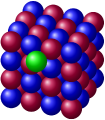
  Протон среди магнитных монополей

• 

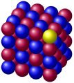
  Позитрон как дырка среди магнитных монополей

• 

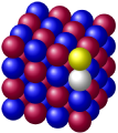
  Электронно-позитронный диполь среди магнитных монополей

• 

  Русская тройка среди магнитных монополей

• 

  Нейтрон как протон, электронно-позитронный диполь и электрон среди магнитных монополей

Априорная теория всего рассматривает только долгоживущие дефекты кристалла из магнитных монополей, необходимые для стабильного функционирования термоядерных реакторов. Тем не менее, некоторые физически осмысленные короткоживущие дефекты могут быть описаны априорной теорией всего как малосущественные детали общей картины.

Долгоживущие дефекты кристаллов хорошо изучены и могут быть использованы в качестве прототипов как уже открытых экспериментально, так и ещё не открытых элементарных частиц. Их совпадение просто поразительно! Прежде всего следует отметить, что и в кристалле из магнитных монополей также существует два типа дефектов, как и в обычных кристаллах.

Дефект по Френкелю — точечный дефекта кристалла, представляющий собой разнесённую пару, состоящую из вакансии (например, электрона или позитрона) и междоузельного протона или антипротона. Образуется в результате перемещения граничного монополя из узла кристаллической решётки в междоузлие (при воздействие на граничный монополь нейтрино и квантов), то есть в такое положение, которое в идеальной решётке монополи не занимают.

Дефект по Шоттки — пара вакансий электрона и позитрона в кристаллической решётке, один из видов точечных дефектов в кристаллах, от дефекта по Френкелю отличается тем, что его образование не сопровождается возникновением междоузельного протона или антипротона. Образуется в результате выхода пары граничных монополей за границу кристалла в реперное пространство. Образовавшаяся при этом пара вакансий затем мигрирует вглубь кристалла. Поскольку образование дефектов Шоттки увеличивает объём кристалла, то, соответственно, плотность кристалла при этом падает. Данный эффект известен в астрофизике как красное смещение.

Электроны и позитроны являются дырками на месте южных или северных монополей. Нейтрон является составной частицей из протона, электронно-позитронный диполя и электрона. Последние три частицы в совокупности удобно называть частицей — русской тройкой.

Наиболее важную роль в создании дефектов играет слабое взаимодействие.

References

АРыбников